Alexander Genser

Problem description

Full paper: | Implementation:

An accurate derivation of fundamental traffic state variables is key for sophisticated traffic management. Urban areas especially suffer from congestion due to a higher population density, traffic lights, and elevated mobility demand. In addition, other variables, traffic flow information at specific locations in the network, and travel times between an origin and a destination are of great importance for traffic operators. In particular, travel times allow for the derivation of the network's current level of service (LoS) and influence the network user's mode and route choice. Consequently, accurate sensor technology is needed to detect vehicles traveling through a network with a low error rate where traffic variables satisfy accuracy requirements [1]. However, urban areas are sometimes sparsely equipped with sensors, which negatively affects accuracy and increases the noise level of the results. In addition, various sensor technologies used in urban environments are only suitable for deriving particular traffic variables and differ in data resolution. New technologies such as video/thermal cameras and Bluetooth/WiFi sensors enable accurate derivation of traffic flow and provide good results in measuring travel time since unique vehicle identification based on MAC address recognition is possible.

Although numerous studies have evaluated and estimated travel times on freeways and in urban areas [2,3,4], only a few studies have compared emerging sensor technologies to empirical ground-truth measurement. In addition, the question remains of how traditional sensor data can help with travel time estimation in terms of performance improvement. Therefore, this work provides traffic state representation regarding traffic flow and travel time estimation within an urban network. We run a multi-sensor campaign in Zurich, Switzerland, including video measurements from a particular area and investigate the time series derivation of travel times. Consequently, we compare the following data sources: (a) thermal camera sensor data that are equipped with a WiFi interface (b) processed video data with an automated license plate recognition (ALPR) algorithm, and (c) Google Distance Matrix data from the particular area. For comparative results, the video data serves for the exact determination of traffic flow and travel times, i.e., a ground-truth data set. Besides assessing the different data sets, we propose a simple yet efficient multiple linear regression (MLR) model to estimate travel times in a future environment with connected and automated vehicles (CAV). We create a baseline scenario with a random 5% sample of the ground-truth data that emulates data from moving sensors (e.g., from CAVs). Finally, a model that fuses moving sensor data with traditional loop detectors (LD) and traffic signal data is proposed. The estimation results are compared to the baseline and ground-truth data.

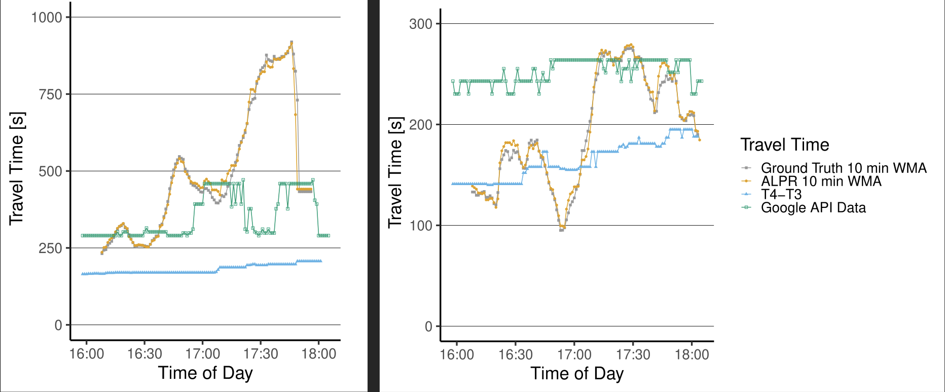
As this study focuses on traffic state estimation via travel time derivation in an urban environment, a small area is selected that reflects the quantities variance but does not allow for complex traffic movements, e.g., a high number of possible routes. The particular area is located in Zurich, Switzerland, in the northern part of the city. A four-leg intersection is selected, where three legs are observed by the given set of sensors. Consequently, six routes are constructed and travel times from the different data sources are determined. The travel time is denoted as τ_i(t), where the index i denotes the route. Figure 1 shows the comparisons of the investigated data sources for route 1 and 5, i.e., τ₁(t), τ₅(t).

The travel time results are derived by determining the timestamp when a vehicle enters and exits the system. As data sources (a) the WiFi module of the installed thermal cameras (in blue), (b) the detected license plates from the ALPR algorithm (in orange) (c) tracked data from the Google Distance Matrix API (in green), and (d) the empirical measurement, i.e., the ground-truth data set (in grey) are used.

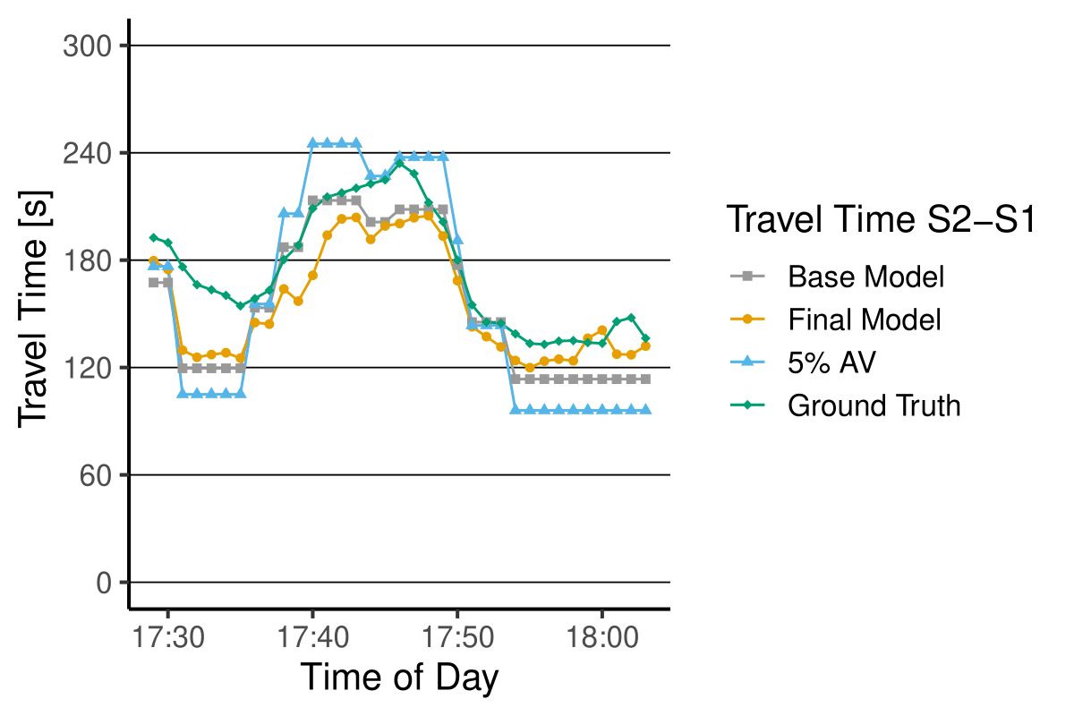
We derive all travel time data sets and calculate the 10 min weighted moving average (the window size k=10). One can note that the quantity τ_i(t) increases over time, peaks around 17:45, and decreases again afterward. Results computed from the ALPR detections (orange time series) replicate this trend with small deviations. The time series correlate with a Pearson correlation coefficient ρ=0.99 and a Mean Absolute Percentage Error (MAPE) MAPE=3.14%. Contrary results are shown by the set of thermal cameras’ WiFi modules that are utilized for travel time derivation of τ_1 (t). The time series only shows small variations and does not capture the trend of the ground-truth data (ρ=0.71;MAPE=58.07%). Potential reasons for the modest performance can be (a) a low penetration rate, i.e., a small number of WiFi devices are detected [5], or (b) the data are strongly post-processed. The time series computed from the Google Distance Matrix API shows a higher variance than the thermal camera data and fails to show the variation of the ground-truth data (ρ=0.27;MAPE=25.95%). For the travel times on r₅, i.e., τ₅(t), the ALPR algorithm allows an accurate representation of the ground-truth data with ρ=0.99 and MAPE=2.73%. The thermal camera data shows a correlation of ρ=0.72 with an MAPE=20.60%, and the Google data allows the computation of ρ=0.33 and MAPE=45.49%. To improve the travel times from data sources as shown above, a estimation methodology is designed that fuses (a) features set computed based on LD data and (b) 5% data sample from Connected Automated Vehicles (CAV) (implemented by drawing a random sample from the ground-truth data). Figure 2 shows results for the test data (30 minute period) and compares (a) the 5% sample, (b) the baseline model (taking just the 5% sample as input) and (c) the final model that fuses the data sources against the ground-truth. Results show that a 5% data sample is insufficient to represent the ground-truth travel time τ₃(t). This is supported by a high MAPE=18.10%. The trained baseline model shows an adjR² of 0.40 and over- and underestimates the travel time in Figure 2. The predicted time series results in an MAPE=11.62%. Nevertheless, it can be shown that our model already improves the estimation by 6.48%. Finally, we apply the model with all features utilized as predictors. Although the model also indicates deviations from the ground-truth data, the adjR² equals 0.81, and the MAPE reduces further to 10.92%. This highlights that the explainability of the final model doubled compared to the baseline model [6].

References

[1] Kouvelas, A.; Chow, A.; Gonzales, E.; Yildirimoglu, M.; Carlson, R.C. Emerging Information and Communication Technologies for Traffic Estimation and Control. Journal of Advanced Transportation 2018.

[2] Bachmann, C.; Roorda, M.J.; Abdulhai, B.; Moshiri, B. Fusing a Bluetooth Traffic Monitoring System With Loop Detector Data for Improved Freeway Traffic Speed Estimation. Journal of Intelligent Transportation Systems 2013, 17, 152–164.

[3] Yildirimoglu, M.; Geroliminis, N. Experienced travel time prediction for congested freeways. Transportation Research Part B: Methodological 2013, 53, 45–63.

[4] Haghani, A.; Hamedi, M.; Sadabadi, K.F.; Young, S.; Tarnoff, P. Data Collection of Freeway Travel Time Ground Truth with Bluetooth Sensors. Transportation Research Record 2010, 2160, 60–68.

[5] Sharifi, E.; Hamedi, M.; Haghani, A.; Sadrsadat, H. Analysis of Vehicle Detection Rate for Bluetooth Traffic Sensors: A Case Study in Maryland and Delaware. 18th ITS World Congress 2011.

[6] Genser, A., Hautle, N., Makridis, M., & Kouvelas, A. (2021). An experimental urban case study with various data sources and a model for traffic estimation. Sensors, 22(1), 144.