Alexander Genser

Problem description

Full paper: | Implementation:

Digitization has substantially transformed the transportation sector over the past decade, providing new data sources (e.g., sensor and in-vehicle technologies) that enable data-driven methods to be integrated into established traffic management systems. Hence, also traffic signal control systems at urban intersections advance (e.g., fully-actuated signal control [1], self- steering algorithms [2]) and affect signal phasing resulting in different green, red, and cycle times.

Therefore, speed advisory systems can benefit if the duration of a future signal phase is known. Ideally, fewer vehicles have to stop when crossing an intersection and uncertainty for other transportation modes is reduced. Signal phasing and timing (SPaT) messages provide the necessary information. Unfortunately, determining the future phase duration of fully-actuated signal control systems is not trivial reverse engineering as predictions depend on Loop Detector (LD) detections that occur after the forecast is applied. Also, such systems typically involve complex optimization, which constitutes a barrier to applying SPaT messages in practice. Therefore, a sophisticated modeling approach using empirical traffic signals and LD data for accurate predictions is still a subject of research.

Contributions

• The framework design allows for predicting the next signal phase of multi-modal fully-actuated signal control systems.
• The prediction of the next red phase, modeled as a supervised learning problem, captures the complex and non-linear relation between a traffic signal and LD detection data.
• The framework requires no prior knowledge about the implemented traffic signal control system.
• A physics-informed feature engineering incorporates the concepts of traffic flow theory. The approach enhances the quality of a given prediction model and can be used for multi-model systems with transit priority.

Findings

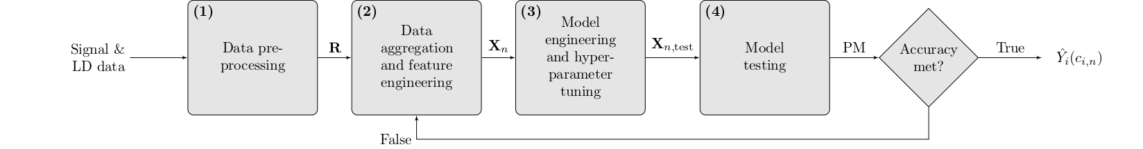
The presented work introduces a T2G prediction framework that allows a generic application to any intersection, providing traffic signal and LD data. The architecture is depicted in Figure 1. The blocks (1) and (3) denote a supervised ML problem’s processing and implementation steps. The raw data (i.e., LD and signal data from the traffic op- erator) functions as an input to the data pre-processing (block (1)). The input signals are transformed into a structured format within this step, and undefined signal states are eliminated. To find out more details about the input data and the corresponding defintion, please check out the project Traffic signal and loop detector data set. Consequently block (2) aggregates and performs the feature engineering to obtain the following list of quantities:

• Red and green time of a given traffic signal
• Traffic flow during red and green time of a given traffic signal, respectively
• The occupancy of a given LD sensor
• The time duration since the last detection of an LD sensor
• A queue and congestion indicator based on longest detection time during a signal phase

The set of features is then utilized to train a set of models (block 3) and determine the best candidate (block 4) for the problem at hand. For this work, a Linear Regression (LR), a Random Forest (RF), and a Long-Short-Term-Memor (LSTM) neural network are assessed against a Naive Baseline model. The full methodology is explained in detail in [3].

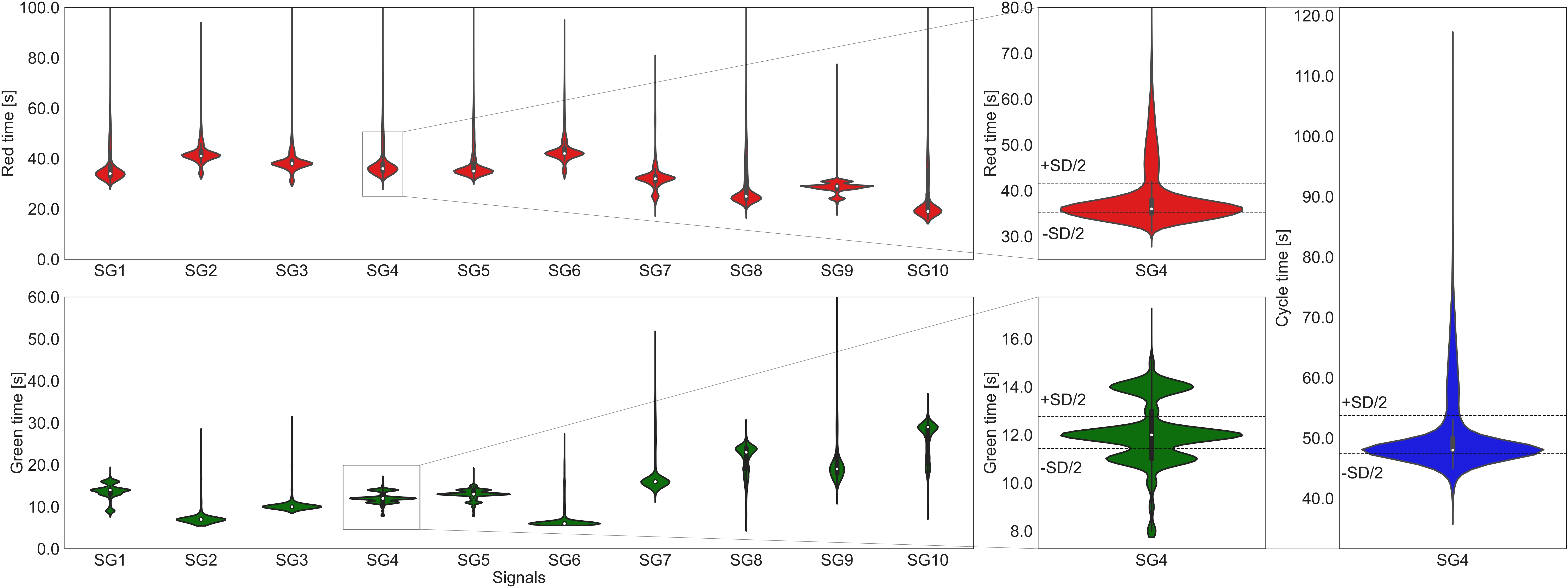
In Figure 2, feature distributions for the red and green times of all traffic signals are presented. The violin plots present the red and green time feature distributions for all considered traffic signals. The data distributions highlight that the signal control system is fully-actuated. For example, the red time of signal 4 (shown separately in Figure 5) operates with an average red time of 38.46 seconds. Nevertheless, the minimum and maximum values in the data set show red times of 29 sec and 104 sec, respectively. Note that signal 4’s red time distribution shows a long tail due to red times higher than 70 seconds. Nevertheless, these samples are not outliers, as the maximum allowed red time for this signal control strategy is fixed to 180 sec. Hence, the prediction models must be capable of learning and predicting this behavior. The threshold values +SD/2 (41.63 sec) and - SD/2 (35.30 sec) highlight the range around the mean value of 38.46 sec. 28207 from 53031 available samples occur within the specified range. Consequently, 24824 samples of signal 4’s red time are outside +SD/2 or -SD/2 and not close to the mean value. This underlines the full actuation of the system and that not just a few samples show a high variance. Similar characteristics can be shown for the green and cycle time distribution of signal 4. The range around the mean green time of 12.01 sec are computed with 12.75 and 11.44 sec. From 53031 samples, 24306 samples are within, and 28725 samples are outside the range between +SD/2 and -SD/2. For the cycle time with a mean value of 50.56 sec, 33323 samples are close to the mean and 19708 samples are outside the range. The descriptive analysis underlines that (a) the system is fully-actuated and (b) a substantial amount of data is different from the mean. Note that signal 4 is presented here as it regulates a traffic stream conflicting with public transportation (controlled by signal 12).

The models on the test data set are assessed with the performance metrics in block (4). First, the Mean Absolute Error (MAE) and the Root Mean Square Error (RMSE) are utilized. Also, two additional and strict error metrics are introduced. To evaluate if the prediction meets the requirements of practical applications (e.g., speed- advisory systems), the work introduces the Exact Hit (EH) and the Near-Misses (NM):

• An EH is defined when the prediction model forecasts the T2G with an error of 0 seconds.
• An NM when the error is lower or equal to two seconds.

The threshold value is chosen based on studies such as e.g., [4], [5], that find the response time for action of Connected Automated Vehicles (CAV) is ranging from one to two seconds (and higher under certain circumstances). Consequently, predictions that are classified as EH or NM can serve as an input to, e.g., motion planning algorithms without forcing a vehicle to stop at an intersection. Note that the T2G values of the test data set are given as integer values; therefore, the prediction values are rounded to integers. Figure 3 shows the final comparison of all models and all performance metrics.

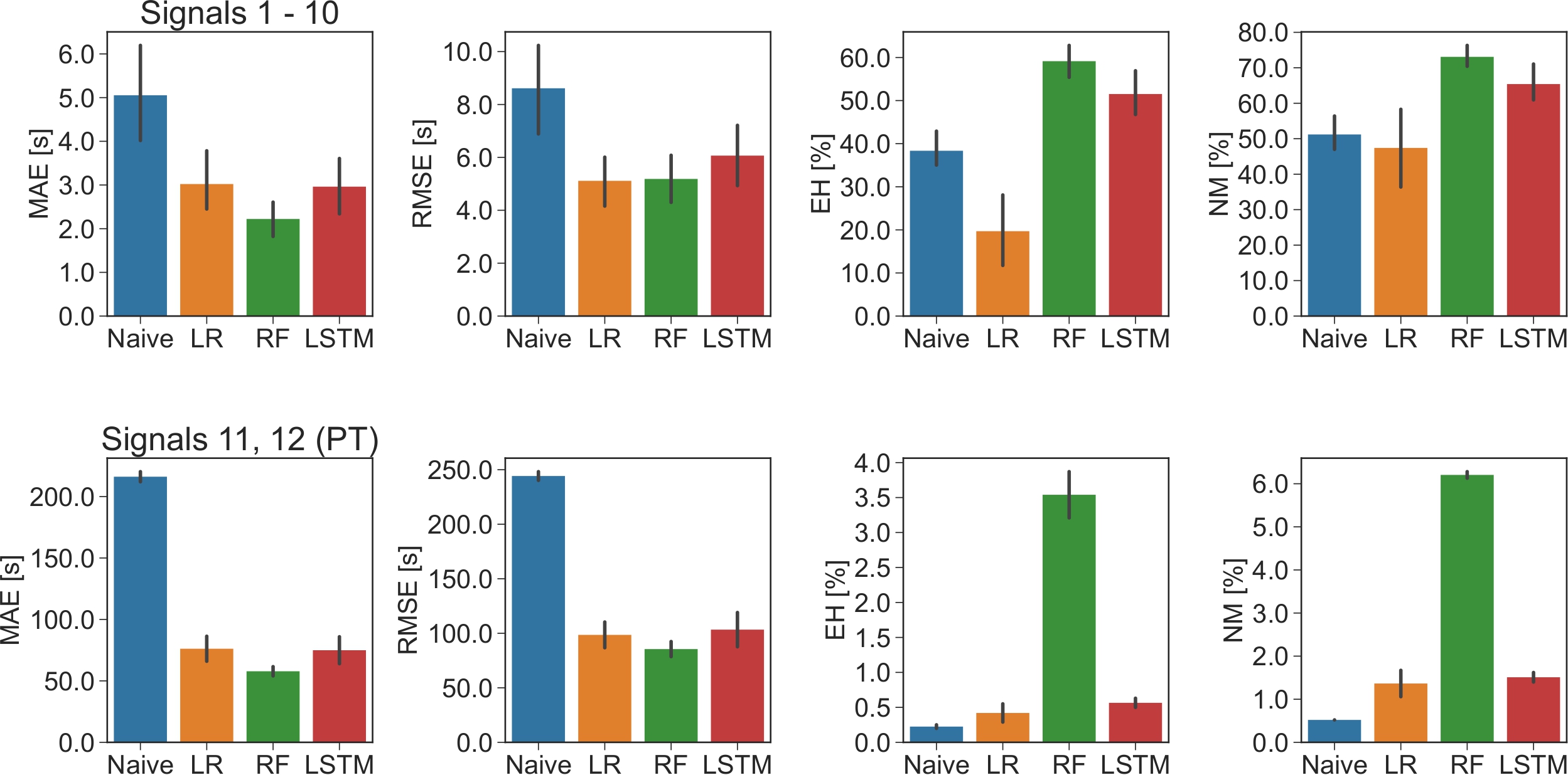
The subplots show the MAE, RMSE, EH, and NM metrics for signals 1 – 10. The RF models show the lowest error values with an MAE of 2.22 sec (standard deviation: 0.66 sec), an EH-ratio of 59.14% (standard deviation: 6.27%), and an NM- ratio of 78.56% (standard deviation: 4.17%). Note that the aggregated RMSE metrics of the LR and RF models show no significant difference with 5.11 and 5.18 sec, respectively.

One advantage of the best candidate in this study is that RFs allow for a straightforward computation of the feature importance. One decision tree in a random forest splits input values based on the condition of impurity. When solving a regression problem, impurity is defined as the variance. When training the model, the weighted impurity should be mini- mized. Each feature’s contribution allows for the calculation of the feature importance to solve the initial problem, i.e., the approximation of a function that maps the input feature vector to the T2G target values. Here the feature importance for the 10 most relevant features for the models of traffic signals 4 is shown. Figure 4 shows the 10 most important features for the prediction of the T2G of traffic signals 4.

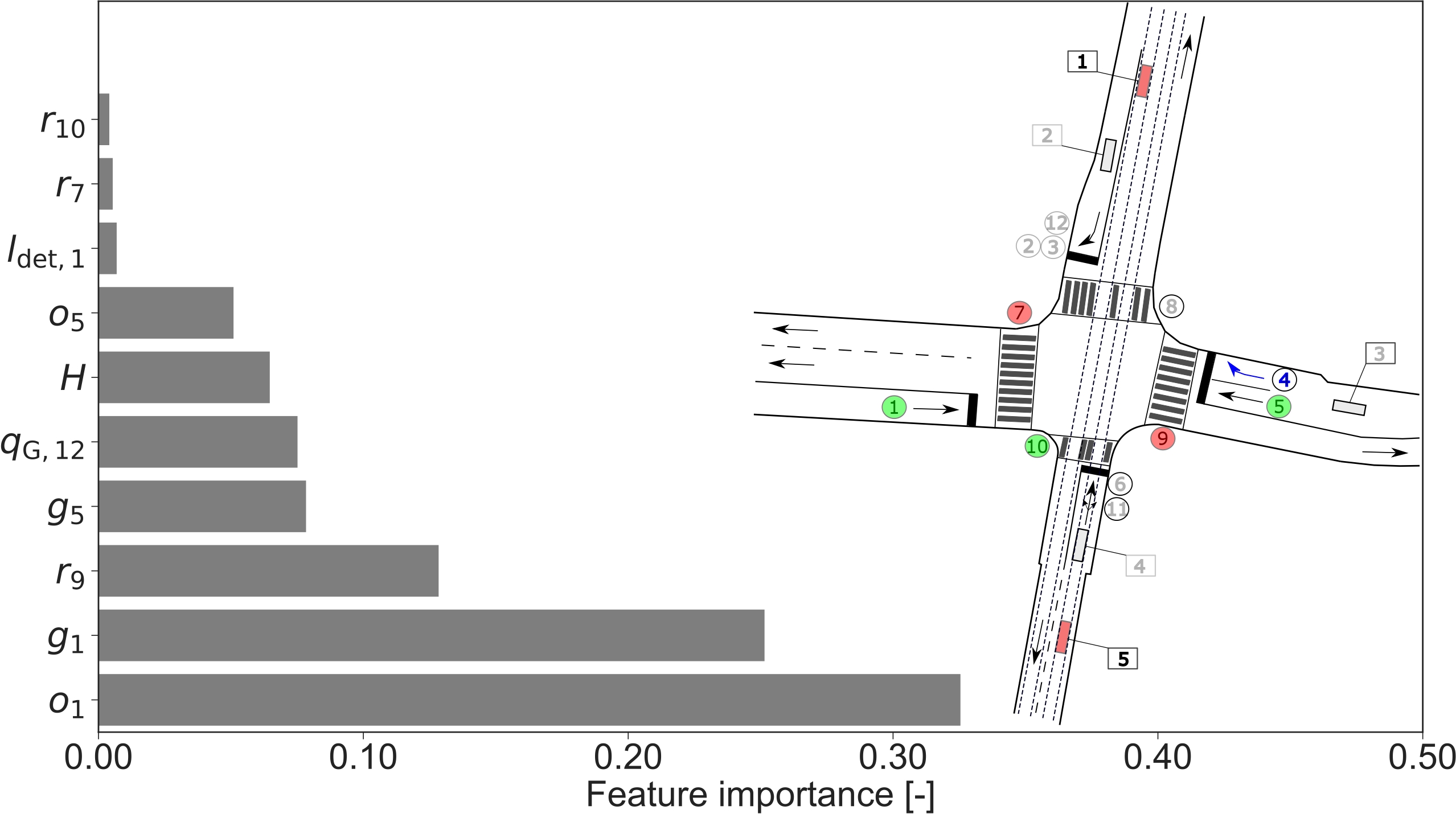
For the both signals, the most important feature appears to be the occupancy of LD 1, i.e., o1 detecting arriving trams from the north of the intersection area. This is expected as the T2G is highly dependent on the priority of public transportation. Additionally, for both models, the occupancy o5 for arriving vehicles and trams from the south is listed in the 10 most relevant features. For the T2G prediction of traffic signal 4, the second most important feature is the green phase’s duration of signal 1, g1 (non-conflicting traffic stream); for the T2G of traffic signal 6, it is the red phase duration, r2. Finally, note that in both cases, the feature representing the hour of the day H is important and highlights that both models find T2G patterns that depend on the time of the day. This result underlines that both data sources are important to determine a prediction of the T2G that meets accuracy requirements. For full results the reader is redirected to [3].

References

[1] X. Zheng and W. Recker, “An adaptive control algorithm for traffic-actuated signals,” Transportation Research Part C: Emerging Technologies, vol. 30, pp. 93–115, 2013.

[2] Lämmer and D. Helbing, “Self-control of traffic lights and vehicle flows in urban road networks,” Journal of Statistical Mechanics: Theory and Experiment, vol. 2008, no. 04, p. P04019, apr 2008.

[3] A. Genser, M. A. Makridis, K. Yang, L. Ambühl, M. Menendez, and A. Kouvelas, "Time-to-Green predictions for fully-actuated signal control systems with supervised learning," arXiv preprint arXiv:2208.11344.

[4] J. S. Brunner, M. A. Makridis, and A. Kouvelas, “Comparing the observable response times of acc and cacc systems,” IEEE Transactions on Intelligent Transportation Systems, pp. 1–10, 2022.

[5] M. Makridis, K. Mattas, B. Ciuffo, F. Re, A. Kriston, F. Minarini, and G. Rognelund, “Empirical study on the properties of adaptive cruise control systems and their impact on traffic flow and string stability,” Transportation Research Record, vol. 2674, no. 4, pp. 471–484, 2020.